Pipe flow

The example in examples/pipeflow/ presents a generic cylindrical straight channel flow scenario that can be the basis for many other projects. The domain considers a single tube, given in tube.stl, with periodicity along the length of the tube, i.e. an endless pipe flow configuration.

The STL file is first voxelised to obtain a discretisation of the pipe domain, after which the periodic boundary conditions are applied. The flow in the domain is driven by applying a homogeneous external body-force, which leads to a Poiseuille flow profile throughout the domain.

The examples considers both red blood cells (RBCs) and platelets (PLTs) of which the initial positions are given in RBC.pos and PLT.pos. To generate alternative initial positions, e.g. using different hematocrit or RBC to PLT ratios, see Cell packing or the packCells tool.

After compilation, the example can be run as:

# run the simulation from the `examples/pipeflow` directory
mpirun -n 1 ./pipeflow config.xml

# generate Paraview compatible output files
../../scripts/batchPostProcess.sh

The initial condition of the pipeflow example. The image illustrates the bounding domain in the black outline, where a cross-section of the fluid field is shown in the solid colors with the initial positions of the red blood cells and platelets (in yellow).

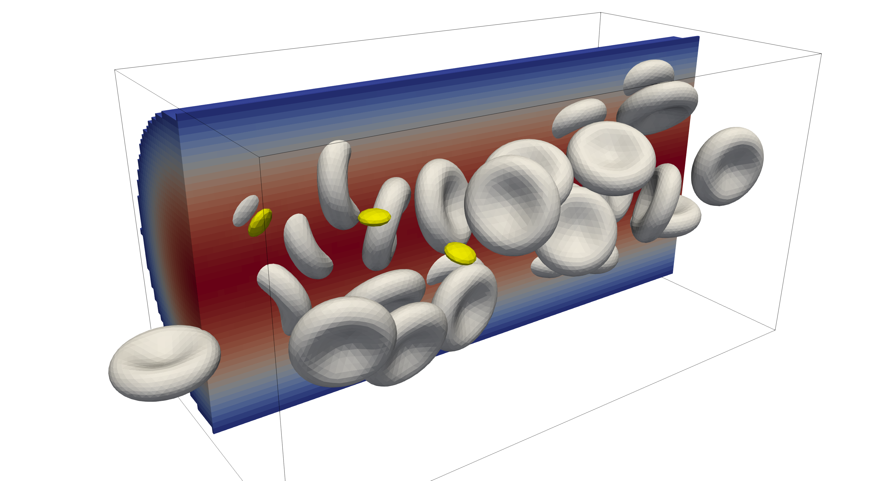
After running for a number of iterations, we can observe the displacements and deformations of the RBCs as the move through the pipe and interact with the available platelets. Note that both the fluid field as well as the particle field show full periodicity along the length of the pipe.

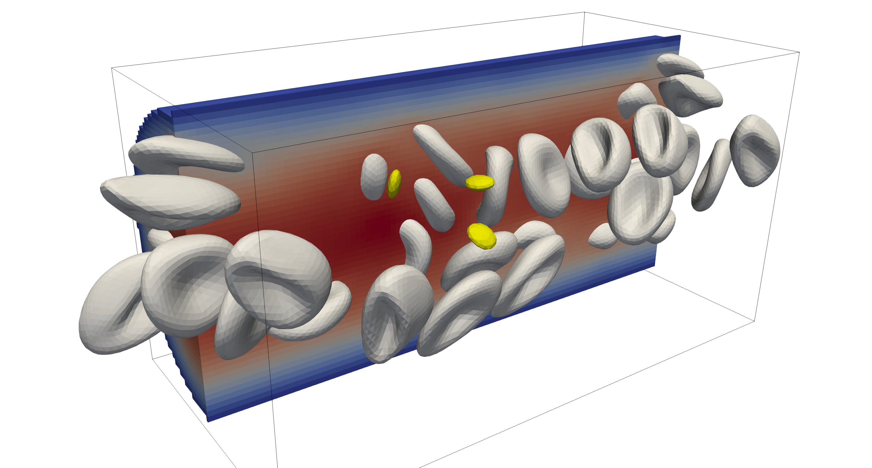
The updated cell positions after various iterations where the displacement and deformations of the particles become visible. In this example a Reynolds number of 0.2 was used.

To change diameter the of the pipe and the initial cell positions, see Configuration.

Configuration

The configuration of the problem is provided in config.xml, where the flow direction through the tube (tube.stl) is assumed aligned with the x-axis. There are three parameters of specific interest for this example

• <domain><refDirN>: this controls the number of fluid cells perpendicular to the flow direction. Thus, this parameter directly controls the diameter of the pipe, as a single fluid cell translates to 0.5µm.

  Note

  When you change the dimensions of the pipe, you might want to update the cell positions accordingly or generate new positions all together, see Cell packing.

• <domain><Re>: the Reynolds force from which the driving for is calculate for the periodic flow through the pipe.

  Note

  The Reynolds number corresponds to the one that would be found when the system is evaluated without any cells present. Thus, the observed velocities might be lower than expected when cells are present in the system. For too larger Reynolds numbers, the simulation might become unstable.

• <domain><geometry>: the STL file used for the discretisation, where tube.stl has been used throughout this example. Other STL files might be used, although care should be taken in modifying the periodic boundary conditions when the inlets of the pipe are changed with respect to the configuration in tube.stl.

Cell packing

The default RBC.pos and PLT.pos files contain many positions for the red blood cells and platelets. The number of particles, their positions, and the ratio between RBC and PLT have all been generated by the packCells tool. For instance, when increasing the size of the pipe, more RBCs and PLTs will fit inside the domain, so you might want to regenerate the initial positions accordingly to populate the pipe with a desired number of particles at the start of the iterations.